Step2. 中級編
1. 2×2のクロス集計表と様々な比率

1-6. コクラン=アーミテージ検定

コクラン=アーミテージ検定は、順序尺度からなる順序データと2値データからなるクロス集計表があるときに、順序データの水準に伴う2値データの傾向性があるかどうかを検定する場合に用います。

例えば、順序データ（ $x_1,\ x_2,\ x_3$ ）と2値データ（ $y_1,\ y_2$ ）からなるクロス集計表の場合、順序データの各水準における $y_1$ の割合（ $a/(a+b),\ c/(c+d),\ e/(e+f)$ ）に直線的な増加もしくは減少の傾向があるかを検定します。

	$y_1$	$y_2$	合計
$x_1$	a	b	a+b
$x_2$	c	d	c+d
$x_3$	e	f	e+f

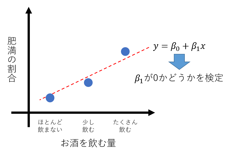
少し分かりにくいので具体例をあげてみます。お酒を「飲まない」、「少し飲む」、「たくさん飲む」人の中で、肥満の割合を調べた結果について考えてみます。

	肥満である	肥満ではない	合計	肥満の割合
お酒を飲まない	10	90	100	10%
お酒を少し飲む	20	60	80	25%
お酒をたくさん飲む	30	30	60	50%

この例では「肥満である」の割合に傾向があるかを検定します。すなわち、X軸にお酒を飲む量の水準を、Y軸に肥満の割合を取ったとったときに、回帰直線の傾きが0でない場合には、お酒を飲む量が増えるにつれて肥満の割合が有意に増加（もしくは減少）すると結論付けられます。

■計算方法

順序尺度からなる順序データ（ $x_1,\ x_2,\ \cdots,\ x_k$ ）と2値データ（ $y_1,\ y_2$ ）からなる次のような結果について考えます。

	$y_1$	$y_2$	合計	割合
$x_1$	$a_1$	$b_1$	$n_1$	$p_1$
$x_2$	$a_2$	$b_2$	$n_2$	$p_2$
︙	︙	︙	︙	︙
$x_k$	$a_k$	$b_k$	$n_k$	$p_k$
合計	$a$	$b$	$n$	$p$

コクラン=アーミテージ検定では、この結果から次のようなカイ二乗値を計算します。 $x_1,\ x_2,\ \cdots,\ x_k$ の値は順序データの値をそのまま使う場合や $1,\ 2,\ \cdots\ k$ という値を用いる場合もあります。

	カイ二乗値	自由度
直線の傾き	$\chi_{slope}$	$1$
直線からのズレ	$\chi_{residual}$	$k-2$
合計	$\chi_{total}$	$k-1$

まず、3つの平方和（ $S_{xx},\ S_{yy},\ S_{xy}$ ）を計算します。

$\displaystyle S_{xx} = \sum_{i=1}^{k} n_i w (x_i-\bar{x})^2$

$\displaystyle S_{yy} = \sum_{i=1}^{k} n_i w (p_i - p)^2$

$\displaystyle S_{xy} = \sum_{i=1}^{k} n_i w (x_i-\bar{x})(p_i - p)$

ただし、 $w$ と $\bar{x}$ は次の式から算出します。

$\displaystyle w = \frac{1}{p(1-p)}$

$\displaystyle \bar{x} = \frac{\sum n_i x_i}{n}$

次に、これらの平方和から各カイ二乗値を計算します。

$\displaystyle \chi^2_{slope} = \frac{S^2_{xy}}{S_{xx}}$

$\displaystyle \chi^2_{total} = S_{yy}$

$\displaystyle \chi^2_{residual} = S_{total} - S_{slope}$

カイ二乗値と自由度から検定を行います。 $\chi^2_{slope}$ を使ったカイ二乗検定の結果が、直線の傾き $\beta_1=0$ であるかどうかの検定結果です。

例題：

上であげたお酒を飲む量と肥満の割合との関係についてまとめた結果を使って、お酒を飲む量に対して肥満の割合に傾向があるかどうかを検証し、結論を導き出してください。有意水準を5%とします。

	肥満である	肥満ではない	合計	肥満の割合
お酒を飲まない	10	90	100	10%
お酒を少し飲む	20	60	80	25%
お酒をたくさん飲む	30	30	60	50%

ここでは、お酒を飲む量の各水準を「お酒を飲まない=1」、「お酒を少し飲む=2」、「お酒をたくさん飲む=3」として計算します。

	肥満である	肥満ではない	合計	肥満の割合
1	10	90	100	10%
2	20	60	80	25%
3	30	30	60	50%
合計	60	180	240	25%

まず、3つの平方和（ $S_{xx},\ S_{yy},\ S_{xy}$ ）を計算します。

$\displaystyle w = \frac{1}{0.25(1-0.25)} = 5.33$

$\displaystyle \bar{x} = \frac{\sum n_i x_i}{n} = \frac{1 \times 100 + 2 \times 80 + 3 \times 60}{240} = \frac{440}{240} = 1.83$

であることから

$\begin{eqnarray*} \displaystyle S_{xx} &=& \sum_{i=1}^{k} n_i w (x_i-\bar{x})^2 \\ &=& 100 \times 5.33(1-1.83)^2 + 80 \times 5.33(2-1.83)^2 + 60 \times 5.33(3-1.83)^2 \\ &=& 817.28 \\ \end{eqnarray*}$

$\begin{eqnarray*} \displaystyle S_{yy} &=& \sum_{i=1}^{k} n_i w (p_i - p)^2 \\ &=& 100 \times 5.33(0.1-0.25)^2 + 80 \times 5.33(0.25-0.25)^2 + 60 \times 5.33(0.5-0.25)^2 \\ &=& 31.98 \\ \end{eqnarray*}$

$\displaystyle S_{xy} &=& \sum_{i=1}^{k} n_i w (x_i-\bar{x})(p_i - p) \\ &=& 100 \times 5.33(1-1.83)(0.1-0.25) + 80 \times 5.33(2-1.83)(0.25-0.25) + 60 \times 5.33(3-1.83)(0.5-0.25) \\ &=& 159.90 \\ \end{eqnarray*}$

となります。これらの平方和から各カイ二乗値を計算すると

$\displaystyle \chi^2_{slope} = \frac{S^2_{xy}}{S_{xx}} = \frac{159.90^2}{817.28} = 31.28$