BellCurveの統計解析ソフトエクセル統計

Step2. 中級編
1. 2×2のクロス集計表と様々な比率

1-2. 検査精度の信頼区間

2×2のクロス集計表から得られた値に対する信頼区間の求め方は、「母比率の信頼区間の求め方」で学んだ方法と同じです。母比率pの95％信頼区間は次の式から求められます。

$\displaystyle \widehat{p}-1.96 \times \sqrt{\frac{\widehat{p}(1-\widehat{p})}{n}} \leq p \leq \widehat{p} + 1.96 \times \sqrt{\frac{\widehat{p}(1-\widehat{p})}{n}}$

この式を見ても分かる通り、サンプルサイズが多いほど95％信頼区間の幅は狭くなります。この式を使って、次のようなデータから「感度」と「特異度」の信頼区間を求めてみます。

	罹患している	罹患していない
検査陽性（＋）	95	3
検査陰性（－）	5	97

■感度：0.95

$\displaystyle 0.95-1.96 \times \sqrt{\frac{0.95(1-0.95)}{100}} \leq sensitivity \leq 0.95 + 1.96 \times \sqrt{\frac{0.95(1-0.95)}{100}}$

$\displaystyle 0.907 \leq sensitivity \leq 0.993$

■特異度：0.97

$\displaystyle 0.97-1.96 \times \sqrt{\frac{0.97(1-0.97)}{100}} \leq specificity \leq 0.97 + 1.96 \times \sqrt{\frac{0.97(1-0.97)}{100}}$

$\displaystyle 0.937 \leq specificity \leq 1.007$

上の式は、「サンプルサイズがある程度大きい場合（目安はnp>5、およびn(1-p)>5と言われています）、二項分布 $B(n,p)$ は正規分布 $N(np, np(1-p))$ に近似できるという定理（ラプラスの定理）」を利用しています。したがって、サンプルサイズが十分に大きくない場合や、標本比率（ここでは感度や特異度）が0や1に近い場合には次の式が用いられる場合があります。nはサンプルサイズ、xはあるイベントの発生回数を表します。

$\displaystyle L \leq p \leq U$

ただし信頼区間の下限値は、次の式から

$\displaystyle L = \frac{x}{x+(n-x+1)F_{1-\alpha/2}(2(n-x+1),2x)}$

信頼区間の上限値は次の式から求めます。

$\displaystyle U = \frac{(x+1)F_{1-\alpha/2}(2(x+1),2(n-x))}{(n-x)+(x+1)F_{1-\alpha/2}(2(x+1),2(n-x))}$

この式は「ClopperとPearsonの正確信頼区間」と呼ばれ、F分布を使って信頼区間を算出します。この式を使って感度と特異度の95％信頼区間を算出すると、次のようになります。

■感度：0.95

n=100、x=95を代入

$\displaystyle 0.887 \leq sensitivity \leq 0.984$

■特異度：0.97

n=100、x=97を代入

$\displaystyle 0.915 \leq specificity \leq 0.994$

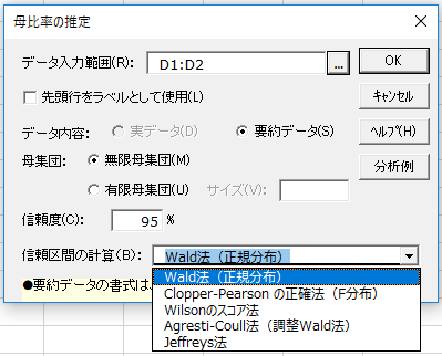
母比率の信頼区間を求める公式は上に挙げた2つ以外にもいくつかの手法があります。エクセル統計には合計5つの手法が搭載されています。

Wald法（正規分布）

Clopper-Pearsonの正確法（F分布）

Wilsonのスコア法

Agresti-Coull法（調整Wald法）

Jeffreys法

また、陽性尤度比と陰性尤度比の95％信頼区間は次の式から算出します。指数関数を使う点がポイントです。

	罹患している	罹患していない	合計
検査陽性（＋）	a	b	a+b
検査陰性（－）	c	d	c+d
合計	a+c	b+d	a+b+c+d

■陽性尤度比：{a/(a+c)}/{b/(b+d)}=感度/{1-特異度}=感度/偽陽性率

$\displaystyle \exp \left[\ln\left(\frac{sensitivity}{1-specificity}\right)\pm 1.96 \sqrt{-\frac{1-sensitivity}{a}+\frac{specificity}{b}} \right]$

■陰性尤度比：{c/(a+c)}/{d/(b+d)}={1-感度}/特異度=偽陰性率/特異度

$\displaystyle \exp \left[\ln\left(\frac{1-sensitivity}{specificity}\right)\pm 1.96 \sqrt{\frac{sensitivity}{c}+\frac{1-specificity}{d}} \right]$

1. 2×2のクロス集計表と様々な比率

統計学やデータ分析を学ぶなら、大人のための統計教室和（なごみ）［業務提携］

オンラインで無料セミナー開催文系のための統計超入門講座

オンラインで学べる集団セミナー統計基礎セミナー（統計検定(R)2級範囲）

【BellCurve監修】統計検定^®2級対策に最適な模擬問題集1～3を各500円（税込）にて販売中！

Kindleストアで配信中

統計検定^®2級模擬問題集1

500円（税込）

統計検定^®2級模擬問題集2

500円（税込）

統計検定^®2級模擬問題集3

500円（税込）